rank函数怎么用（ExcelRANK函数介绍）

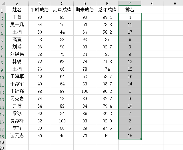
在我们身边经常遇到给Excel里的数据排名，如给下图的表格名单排名

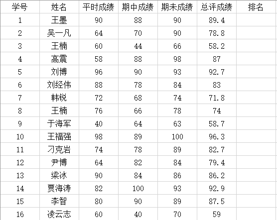
我们一般方法先给总评成绩这列从大到小排序，再给排名那列输入1、2并自动填充完，再把学号这列从小到大排序来完成排名。

今天教大家利用RANK函数轻松完成排名。

先来认识RANK函数：

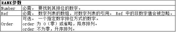
RANK(number,ref,[order])

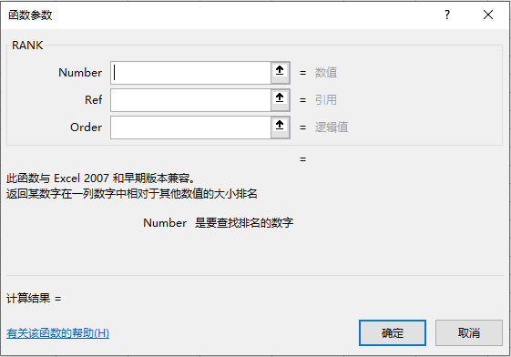
函数对话框：

使用方法：

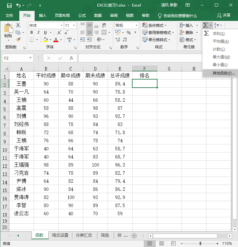
函数调用方法：第一步：点击要排名的那个单元格，再点击开始功能选项卡里的编辑里的自动求和下的其它函数。

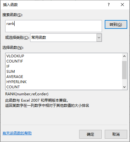
第二步：在插入函数对话框的搜索函数栏里输入rank，点击“转到”出现rank函数后点确定按钮

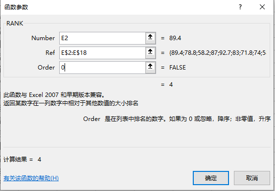
第三步：在函数参数对话框里，Number栏里输入“E2”,在Ref栏里输入"E$2:E$18",在order栏里输入0（可以不输入），并点“确定”按钮

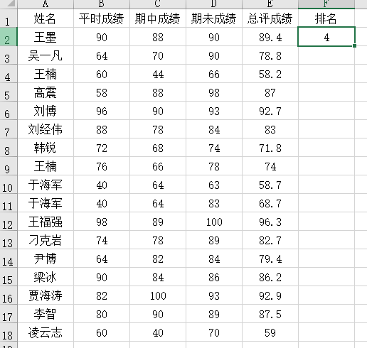
此时已经把第二行“王墨”的总评分数排名就出现了

第四步：f2到F18利用自动填充功能自动求出排名（开始功能选项卡里的编辑里的填充下的向下填充来自动填充。）

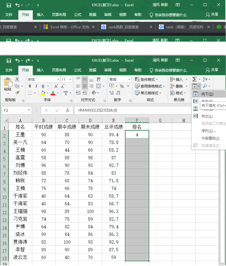
注意：为什么在Ref栏里输入"E$2:E$18"的行号里输入$，目的是E$2:E&18不会因为自动向下填而改变Ref引用的地址的行号变化。